Points as Tori: Fast Pointwise Signed Distance for Point Clouds
ACM Transactions On Graphics (SIGGRAPH 2026)
\(^\dagger\) indicates equal contribution
Abstract
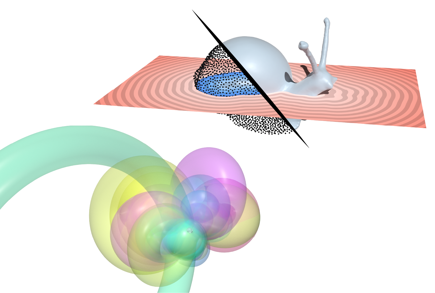
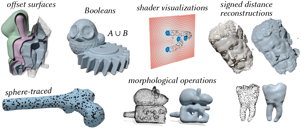
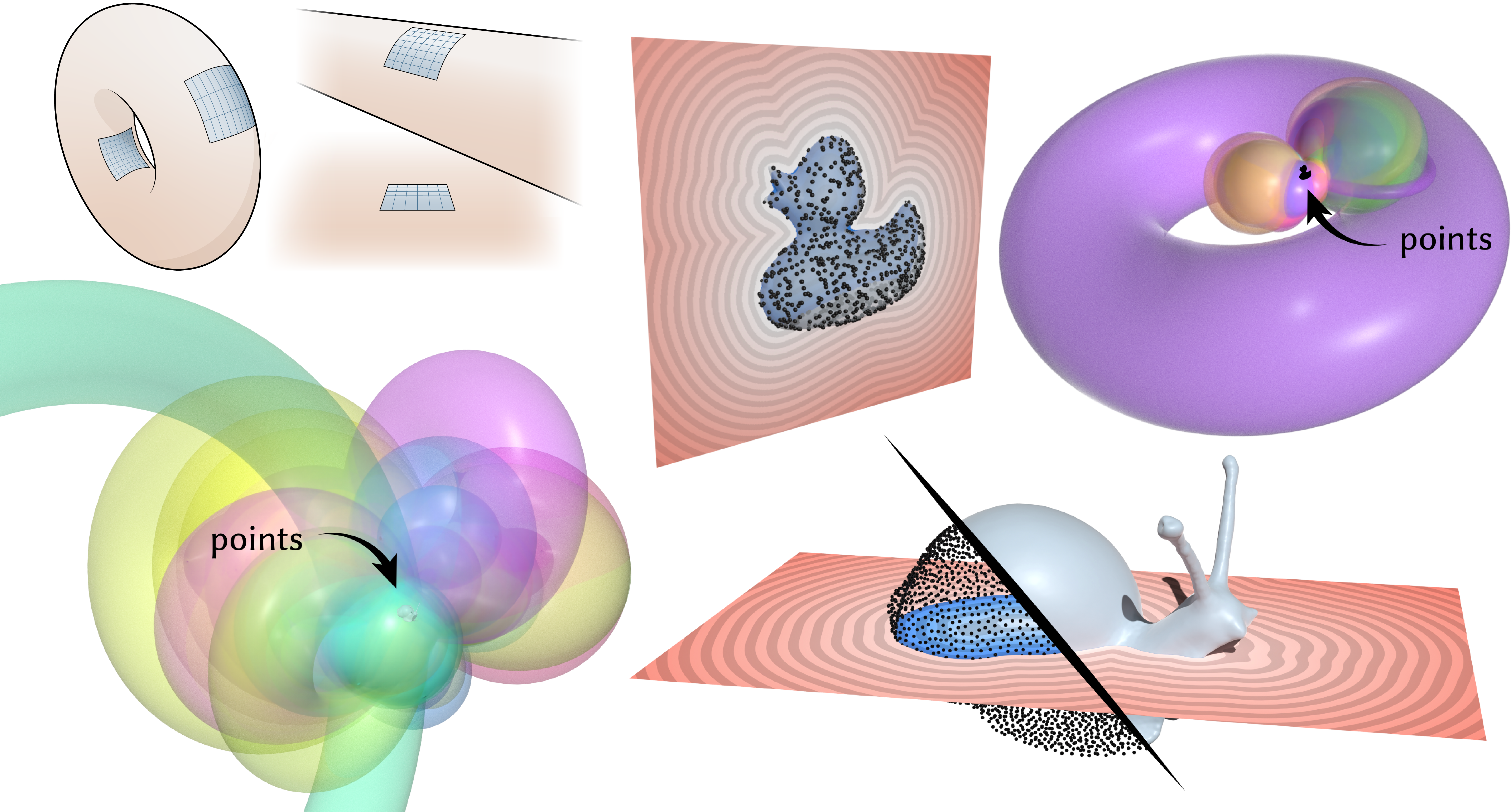
We describe a method for computing signed distance to point clouds that allows fast pointwise evaluation at arbitrary spatial resolution. As input, our method takes a point cloud with normals; as output, it provides an analytical parameterization that allows queries of signed distance to the approximate underlying surface at arbitrary points — simultaneously providing reconstruction and distance. Our key idea is to reconstruct shapes by locally fitting point clouds with tori, which have closed-form signed distance functions. Tori are fitted in a feed-forward manner, using a pre-trained network to output per-point curvature and shift parameters. Importantly, our method does not require costly global optimization or spatial discretization, and is easily parallelizable. Underlying our method is a new theory that unifies signed distance with the classic reconstruction methods of winding numbers and Poisson surface reconstruction. We use our method to compute signed distance to point clouds arising from photogrammetry, meshes, 3D Gaussians, and neural implicits. Our method allows point clouds to be used directly in applications, without explicit surface reconstruction: as examples, we take offsets of point clouds, apply morphological and Boolean operations, and directly visualize offset surfaces using sphere tracing.

- Coming in July
Acknowledgements
This work was funded by NSF awards 2047341, 2212290 and 2504890, and a gift from nTopology. The authors thank Alexander Belyaev and Pierre Fayolle for inspiring conversations about distance computation; Chris Wojtan, Christian Hafner, Samara Ren, Aleksei Kalinov, and Mikaël Ly for helpful discussion; Rohan Sawhney and Josua Sassen for discussion of early ideas; and Hanyu Chen and Benran Hu for providing point cloud data.Fast Forward
To be presented in JulyTalk at SIGGRAPH 2026
To be presented in July To be presented in July
Errata
In the original version of the paper, I unfortunately misspelled Anand Rangarajan's name in Figures 5 and 6. This has been corrected in the version on my website.What is this paper about?
This paper introduces a method called points as tori (PAT) for computing signed distance to point clouds, that allows fast pointwise evaluation of signed distance at arbitrary spatial resolution, without requiring discretization, global optimization, or explicit reconstruction.
In a nutshell, signed distance computation has been either fast or robust (i.e. able to generalize from imperfect shape observations like point clouds) — but not both. We explain why, and develop a simple algorithm that directly estimates signed distance from point clouds.
In the end, given a point cloud with normals \(P = \{(\mathbf{p}_i, \mathbf{n}_i)\}_{i=1}^{|P|}\), our method evaluates signed distance \(\phi(\mathbf{x})\) at a given point \(\mathbf{x}\in\mathbb{R}^3\) simply using the kernel density estimator \[\phi(\mathbf{x}) = \frac{\sum_{i=1}^{|P|} g_i(\mathbf{x}) \exp\left(-\lambda_{\mathbf{x}}\|\mathbf{x}-\mathbf{p}_i\|\right)}{\sum_{i=1}^{|P|} \exp\left(-\lambda_{\mathbf{x}}\|\mathbf{x}-\mathbf{p}_i\|\right)}, \hspace{1cm} (1)\] giving an exponentially-weighted average of per-point functions \(g_i\) associated with each point. We define \(g_i\) as signed distance functions (SDFs) of tori, because torus SDFs have efficient closed-form expressions, and tori can locally approximate surfaces up to second order. The parameter \(\lambda_{\mathbf{x}}\) is automatically chosen with a simple expression. Variants of Equation 1 have been used as heuristics in other point set methods, but were underexplored for signed distance.
The main challenge in our method is fitting tori to a given point cloud \(P\), and we determine these tori by pre-training a neural network to learn surface parameters that give good signed distance to point clouds. This network takes as input a size-\(k\) neighborhood of a point \(\mathbf{p}_i\), and returns parameters yielding a "best-fit" torus intended to provide a good signed distance reconstruction of the point cloud. Once this network is trained, one can infer signed distance from *any* point cloud.
Why this formulation?
In a rare instance, I actually think the explanation is best understood by reading the paper (specifically Section 2).
But in summary, we show that there are two deterministic, single-pass formulas for approximating distance to a surface \(\Omega\), called convolutional distance formulas: the first has the general form \[ \widetilde{d^\lambda}(\mathbf{x}) = -\frac{1}{\lambda}\log\left(\int_\Omega h(\mathbf{x}, \mathbf{z})\exp\left(-\lambda\|\mathbf{x}-\mathbf{z}\|\right)\ \mathrm{d} A(\mathbf{z})\right) \hspace{1cm} (2) \] and can be derived either via a Hopf-Cole transformation of an eikonal equation, or via Laplace's method. This formula subsumes many (unsigned) distance approximations such as LogSumExp distance [Madan and Levin 2022], the Kreisselmeier-Steinhauser function [Kreisselmeier and Steinhauser 1980], Varadhan's formula [Varadhan 1967], and the Schrödinger distance transform [Gurumoorthy and Rangarajan 2009] as special cases. We also show how this formula unifies signed distance with the popular reconstruction methods of (regularized) winding numbers [Jacobson et al. 2013, Chen et al. 2024] and Poisson surface reconstruction [Kazhdan et al. 2006].
As \(\lambda\to 0\), the function \(w\) converges to a jump harmonic function describing inside-outside (left). As \(\lambda\) increases, \(w\) converges to a signed distance function via a log transformation (right). However, we also show this formula works only for closed geometry, and fails for sampled geometry like point clouds.
Unfortunately, convolutional distance approximations are essentially single-point approximations, which makes them not capable of generalization by nature:
 In particular, one obtains a distance function whose level sets are to the sampled geometry, rather than to the underlying surface from which the discrete geometry is sampled. And, as discussed further in the paper, there is little one can do to regularize this function while still preserving distance properties. So while the derivations are elegant and unify decades of geometry processing algorithms (in reconstruction, implicit modeling, distance, point set methods, etc.), the analysis also shows that none of these many dozens of past approaches can provide generalized distance from point clouds (no matter how beautiful the story would have sounded!)
Under this framework, one can also derive a self-normalized convolutional formula (terminology we take from Belyaev and Fayolle [2024]) \[ \widehat{d^\lambda}(\mathbf{x}) = \frac{\int_\Omega g(\mathbf{x},\mathbf{z})\exp\left(-\lambda\|\mathbf{x}-\mathbf{z}\|\right) \ \mathrm{d} A(\mathbf{z})}{\int_\Omega \exp\left(-\lambda\|\mathbf{x}-\mathbf{z}\|\right)\ \mathrm{d} A(\mathbf{z})} \hspace{1cm} (3) \] that gives a smooth approximation of the minimum of \(g\) as \(\lambda\to\infty\). Uses of this formula include kernel regression, partition-of-unity methods, the induced exponential function, the softmax function, etc. Naively, this formula also exhibits similar drawbacks as Equation 2. But the self-normalized variant holds more promise because we can control the estimated manifold's landscape at the closest point via the functions \(g\), whose effective design space is much larger. In particular, we use the SDFs of tori, which, unlike other second-order surfaces like quadratic polynomial patches or quadric surfaces, admit inexpensive, closed-form signed distance queries.
In the end, the most effective approach (out of many that we tried) boiled down to this deceptively simple idea of interpolating local estimates.
Why learning?
Fitting a torus to a given (smooth) surface is easy; the hard part is getting the surface in the first place. Inferring the true surface underlying a point cloud, even locally within a small neighborhood is difficult, because just figuring out what this neighborhood should be is really difficult. Classic methods are extremely dependent on heuristics for neighborhood size and shape. For example, a classic paradigm is to use a Gaussian kernel to determine neighborhood size, which we find incredibly brittle: there's no one kernel bandwidth that yields good results, and so the downstream SDF breaks down.
Because of how difficult this problem is, there has been a *huge* amount of literature proposing endless variations of similar kernel-based methods for (local) reconstruction. Unfortunately, there often is no easy answer: especially around edges, corners, etc., defining neighborhoods is a chicken-and-egg problem, and classical hierarchical approaches/anisotropic kernels still proved brittle; robust estimators/iterative solvers are expensive (see Section 4.4 of the paper for more discussion). So, rather than than manually tweak the parameters of one particular surface-fitting model, we decided to simply use fixed-size neighborhoods with a data-driven approach that can fit to large sets of (easy-to-generate) examples — a far more sophisticated data-fitting model than we could ever craft purely by hand.
Still, the network is fairly lightweight by modern standards: pre-training took about 45 hours on a single GPU (NVIDIA RTX 3090), and the network takes about 6.4MB on disk. We can design and train this network easily, precisely because we've broken down the problem into one that is dominated by local surface behavior.
Why not end-to-end learning?
In contrast to other learning-based approaches that try to directly learn SDFs from entire point clouds, we intentionally invoke the minimum amount of learning needed. We rely on classical results for convergence to true signed distance, and using learning only for the one component with no easy analytical solution.
In practice, learning SDFs end-to-end is also difficult because the eikonal equation \(\|\nabla\phi\|^2=1\) is nonlinear and has many local minima, and function values depend nonlinearly on neural network parameters. Many neural SDF-based methods also fit a neural network to a given shape; in other words, they must train a new network for every shape. In contrast, our method completely sidesteps the difficulties of fitting neural fields to the eikonal equation — and the issues of expensive per-shape training, expensive inference, and limited scalability — by formulating signed distance reconstruction as a purely local problem, before applying a simple analytical formula to produce distance. The result is less training (the network shares weights across point neighborhoods, across all shapes, so needs only one-time pretraining), and ultimately, faster inference time.
Discussion
Commentary that didn't fit in the paper. This section is "for experts only": this section discusses finer technical details, and you certainly don't need to understand this section to understand the paper.
Connection to the signed heat method
My previous project developed the signed heat method (SHM) for "generalized" signed distance: the method computes distance to a nice surface reconstruction (completion) of a noisy, hole-y, etc. set of shape observations, including point clouds.
The signed heat method (and its sibling, the vector heat method) actually already implements a version of Equation 3 on surfaces, where the function \(g\) corresponds to vector-valued data. (The signed heat method, because it diffuses normal vectors, in principle can also exhibit the same artifacts as naive linear, "pseudonormal"-based completion, but its discretization and global integration step helps smooth/average this out.)
Naive convolutional distance formulas (Equations 2 and 3) cannot give both a good reconstruction and good distance, because the parameter \(\lambda\) is coupled to both in opposite directions. The signed heat method essentially decouples these two things by diffusing vectors (rather than scalar-valued data) and its intermediate normalization step. Actually, the diffused vectors before normalization still exhibit the short-time diffusion-based phenomenon of being really concentrated around the points (see figure below) but the method works because the concentration is instead happening in the magnitude of the vectors — the vectors still have the right direction. This behavior is significantly different than diffusing scalar data, where it's hard to get a generalized distance function because the concentration is happening directly in the scalar function that we care about.
Unfortunately, directly adapting the signed heat method to support efficient pointwise queries proves extremely difficult. At first, it appears the signed heat method boils down to solving the Poisson problem \(\Delta\phi=\nabla\cdot Y_t\) , where \(Y_t := X_t/\|X_t\|\) is the normalized version of the vector field solution obtained from the SHM's initial vector diffusion step. It’s tempting to turn this Poisson equation into its corresponding integral equation to gain the computational flexibility we ask for, but the resulting integral is ill-posed.
As a concrete demonstration, consider a sphere of radius \(R\) centered at the origin in \(\mathbb{R}^3\), which has signed distance function \(\phi(x)=\|x\|-R\). The gradient of \(\phi\) is \(Y(x)=x/\|x\|\), and the divergence of \(Y\) is \((\nabla\cdot Y)(x)=2/\|x\|\).
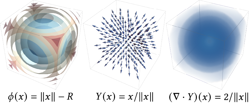
One can verify that attempting to integrate \[\phi(x)\overset{!}{=}\int_{\mathbb{R}^3} G(x,y)(\nabla\cdot Y)(y)\mathrm{d}y\] yields \(\infty\). The divergence \(\nabla\cdot Y\) decays too slowly, and Green's representation formula can only be extended to infinite regions if the solution decays to zero at infinity [Brebbia et al. 1984, §2.10] — whereas a distance function goes to infinity at infinity.
Likewise, the integral equation corresponding a to a finite domain \(M\) \[\phi(x) = \int_{\partial M} \left[\frac{\partial G_M(x,z)}{\partial n(z)}\phi(z) - G(x,z)\frac{\partial\phi}{\partial n(z)}\right]\mathrm{d}z + \int_M G(x,y)(\nabla\cdot Y_t)(y)\mathrm{d}y,\] using an appropriate fundamental solution \(G_M(x,y)\), is recursive in \(\phi\): the first term requires we know the value of the solution \(\phi\) on the domain boundary \(\partial M\). (In contrast, convolutional distance formulas do exist as boundary integrals, because through exponentiation the solution does have proper decay at infinity.)
So in summary, it is not easily possible to remove or change the integration step of the signed heat method (mapping a vector field to a scalar function). Compared to the current method, the SHM tends to have less failure when given point clouds that are severely "out of distribution" (different than data seen in training), but you pay more with each application of the method. In this method, you pay more up front (via pretraining), and get much better performance on in-distribution data.
Connection to kernel methods
Section 3.2 of the paper extensively discusses the connection of our method to other kernel methods, including past convolutional distance formulas, implicit modeling, and manifold learning techniques. A theme of our analysis is that while exponential asymptotics are useful for clustering problems, they are often detrimental in regression problems.
One class of regression problems where exponential asymptotics really hurt are generative models. "Flow-based" generative models in particular aim to sample from a target probability distribution by transforming samples from some easy-to-sample distribution. This transformation is usually parameterized as a time-dependent differential equation, and actually has a simple, closed-form solution that gradually pushes samples towards the closest datapoint seen in training. Hence flow-based generative models such as diffusion models and flow matching amount to simple kernel regression formulas based on Equation 3 [Scarvelis et al. 2023; Gao and Li 2024; Kamb and Ganguli 2025]. This means they can only "memorize" their training data, simply reproducing the discrete training distribution rather than the true distribution from which the training data is sampled — exactly the phenomenon underlying the fundamental limitation of naive convolutional distance formulas.
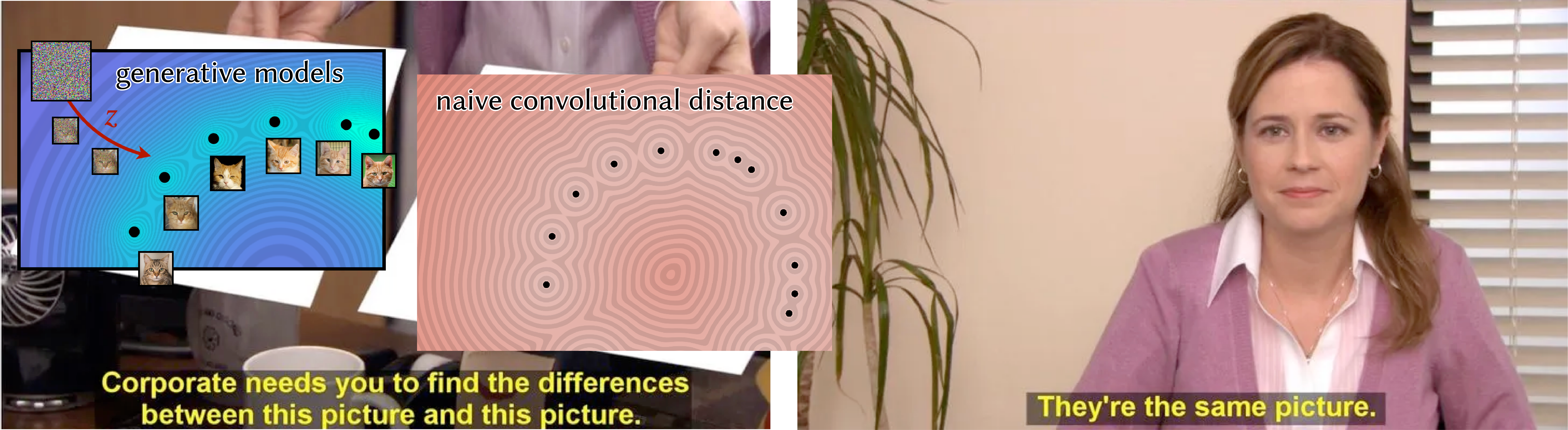
Flow-based models simply reproduce the distribution represented by the discrete training data, rather than the true distribution that we hope to approximate. This is exactly the reason why naive convolutional distance formulas all fail to generalize.
The observation about the "memorization-generalization tradeoff" in the context of generative models has been made by many authors [Liu et al. 2022; Somepalli et al. 2022; Pidstrigach 2022; Yoon et al. 2023; Carlini et al. 2023; Jain et al. 2024; Gu et al. 2025; Biroli et al. 2024]. The current state-of-the-art achieves generalization by instead training expensive neural networks to approximate the score function, rather than using the closed-form formula: generalization doesn't come from the actual flow model, but rather from the neural network (over)regularizing the score function. Scarvelis et al. 2023 develop a closed-form generative model by regularizing the kernel in a manner reminiscent of Chen et al. 2024, though adding noise to the model can easily lead to lower-quality output [Arjovsky et al. 2017]. Recent geometry-based approaches to generative modeling include Bamberger et al. 2025 and Wang et al. 2026.
Limitations and next steps
Section 6 of the paper discusses eight or nine possible lines of future work and improvement, ranging from accelerating precomputation, to further developing our points-as-tori shape representation as a tool for differentiable optimization or compression.