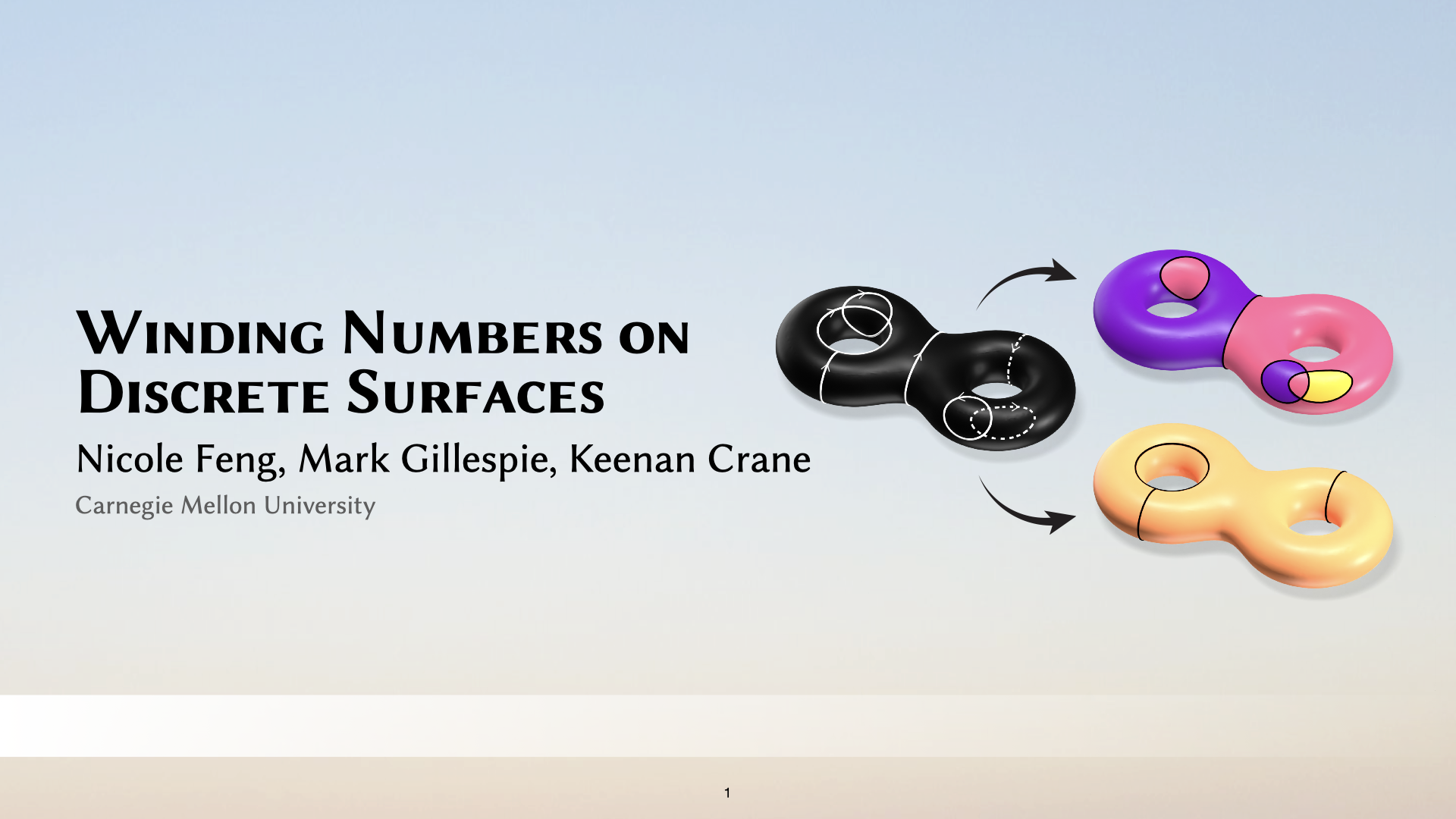
Winding Numbers on Discrete Surfaces
ACM Transactions On Graphics (SIGGRAPH 2023)
Abstract
In the plane, the winding number is the number of times a curve wraps around a given point. Winding numbers are a basic component of geometric algorithms such as point-in-polygon tests, and their generalization to data with noise or topological errors has proven valuable for geometry processing tasks ranging from surface reconstruction to mesh booleans. However, standard definitions do not immediately apply on surfaces, where not all curves bound regions. We develop a meaningful generalization, starting with the well-known relationship between winding numbers and harmonic functions. By processing the derivatives of such functions, we can robustly filter out components of the input that do not bound any region. Ultimately, our algorithm yields (i) a closed, completed version of the input curves, (ii) integer labels for regions that are meaningfully bounded by these curves, and (iii) the complementary curves that do not bound any region. The main computational cost is solving a standard Poisson equation, or for surfaces with nontrivial topology, a sparse linear program. We also introduce special basis functions to represent singularities that naturally occur at endpoints of open curves.
Perspectives on Winding Numbers (supplemental, 2.7mb)
A discussion of different mathematical and physical interpretations of winding number.

A C++ implementation of surface winding numbers (SWN).
For SIGGRAPH poster session.
Social media
Acknowledgements
This work was funded by an NSF CAREER Award (IIS 1943123), NSF Award IIS 2212290, a Packard Fellowship and gifts from Facebook Reality Labs, and Google, Inc.Fast Forward
Talk at SIGGRAPH 2023

What problem does this paper solve?
For a given point on a surface, we would like to know whether it is inside or outside a given curve. For example, coloring points on this cow according to inside vs. outside would look like this:
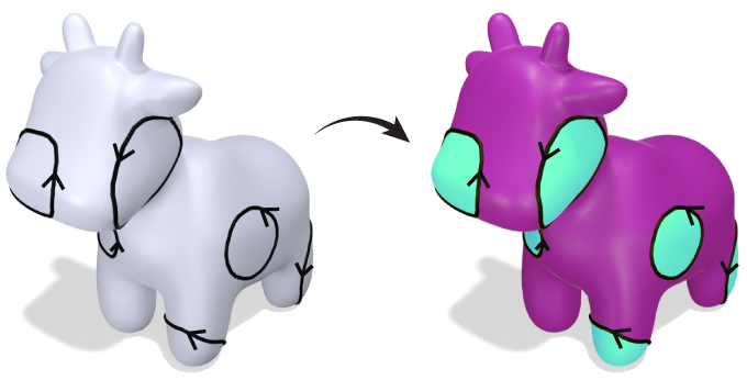
But on surfaces, not all closed curves bound regions:
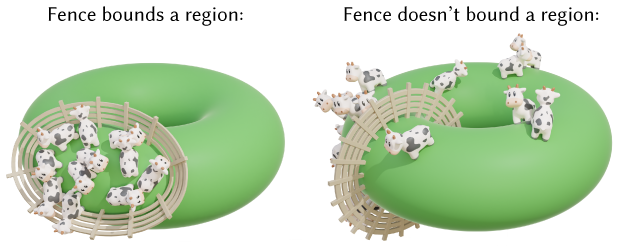
On the left, a fence on Planet Cow forms a closed curve, and the cows are confined to one region. But the fence on the right also forms a closed curve with no gaps, and yet the cows are free to roam wherever they'd like. (Figure idea from Mark Gillespie!)
We'll call curves like the one on the left bounding, because they bound a region, and curves like the one on the right nonbounding because they don't bound regions. So far, we've established that while inside/outside is not well-defined for nonbounding curves, inside/outside is at least well-defined for bounding curves.
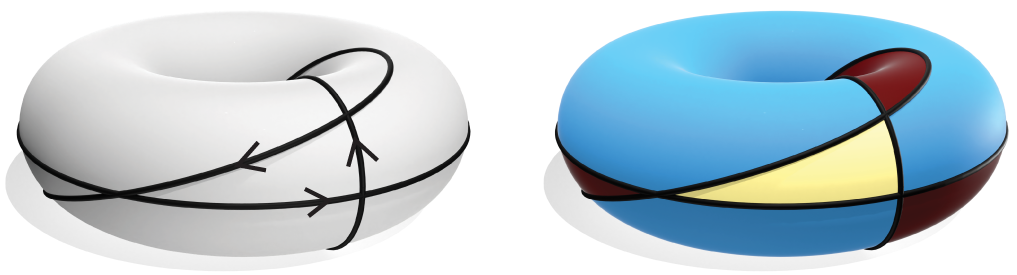
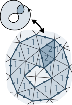
However, an algorithm for computing inside/outside is not so simple as classifying loops as "bounding" vs. "nonbounding", since nonbounding loops can combine to bound valid regions (figure reproduced from Riso et al. 2022, Fig. 4):
More generally, there are numerous ways inside/outside can fail to be well-defined if we're willing to consider all types of surface domains, in addition to those that are multiply-connected:
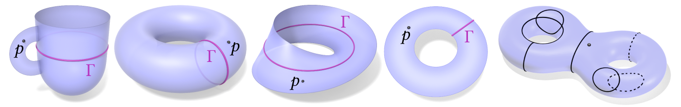
Computing inside/outside gets even harder if some of the curves have been corrupted somehow and are now "broken", for example the "dashed" curves in the rightmost example above, which represent partial observations of an originally whole curve. We would like to answer "inside or outside?" for the point \(p\) in all of the examples shown above.
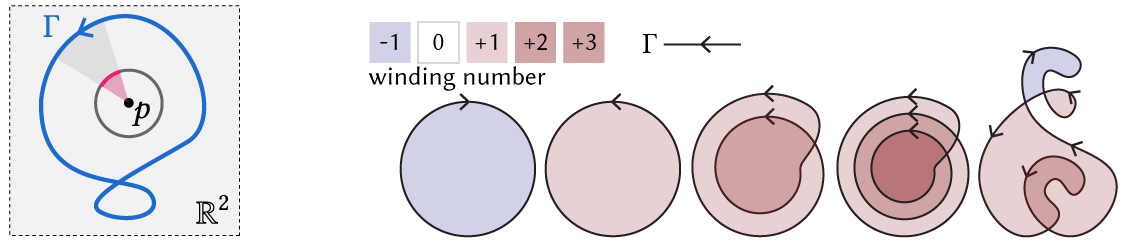
Our starting point to reasoning about all of the above is the winding number, a quantity which appears widely across math and physics. Intuitively, the winding number at a point \(p\) measures the infinitesimal angle subtended by the curve at \(p\), and sums up all these angles over the curve. For a closed curve in the plane, this gives us a piecewise constant function whose value at each point tells us how many times the curve "winds" around it. Hence winding number is fundamentally a topological quantity (though it is often defined through a geometric formula). One can also consider a generalization of winding number called solid angle, which considers open curves in addition to closed curves.
Researchers in computer graphics and geometry processing have in fact already used the properties of solid angle in other works. Perhaps the most well known examples are the equivalent* methods of Poisson Surface Reconstruction [Kazhdan et al. 2006] and generalized winding number [Jacobson et al. 2013] (*see Chen et al. 2024 for a precise explanation of the equivalence). However, all past methods are only applicable to Euclidean domains like \(\mathbb{R}^n\), not general surface domains. For deeper discussion of why usual interpretations of solid angle don't apply in surface domains, see our supplemental, "Perspectives on Winding Numbers".
At the time of our work, there had been relatively little mathematical or algorithmic treatment of winding number on surfaces. Riso et al. 2022 had recently developed the algorithm "BoolSurf" for computing booleans on surfaces — but assumed that the input curves are closed, and already partitioned into loops. It remained an open question of how one could optimally infer the curve's topology from unstructured input. More generally, we aimed for a principled handling of surfaces with boundary, and other types of surfaces.
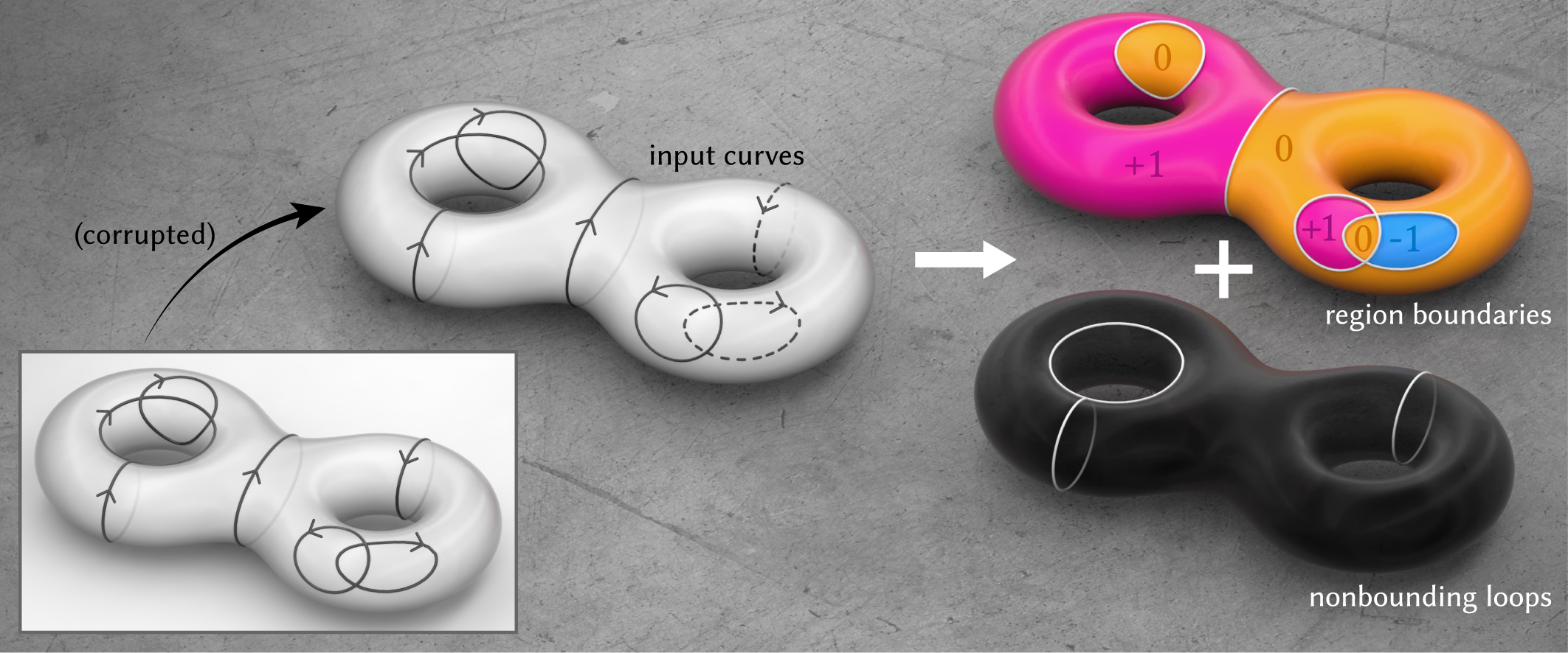
Concretely, our algorithm does the following: Given an unorganized collection of curves with orientations -- meaning each curve has a specified direction from one endpoint to the other, but otherwise with no additional structure -- we determine inside vs. outside on general surfaces. Importantly, we do so robustly, meaning the algorithm reliably outputs correct answers even in the presence of noise and errors. In the process, we determine the bounding vs. nonbounding components of the curve, and produce a closed, completed version of the input curve.
In short, we obtain an algorithm that answers the fundamental question of inside/outside. In turn, the algorithm can form a basic building block of many geometry processing tasks ranging from region selection to curve completion to boolean operations on shapes.
An example of using our algorithm to compute boolean operations between regions defined by imperfect, broken curves.
How does the paper solve the problem?
In a nutshell: the key idea of our method is to turn the harder problem of determining inside/outside of arbitrary curves, into an easier, but equivalent problem about vector fields.
As mentioned earlier, we start from the established concept of winding number. Ordinary winding number is often presented as an integral: for example, in differential geometry, the winding number \(w_\Gamma(x)\) of a curve \(\Gamma\) at a point \(x\in\mathbb{R}^2\) is usually defined as \(w_\Gamma(x)=\frac{1}{2\pi}\int_\Gamma \frac{\langle n_\Gamma(y), y-x\rangle}{\|x-y\|^2} {\rm d}y \), or equivalently in complex analysis as the complex contour integral \(w_\Gamma^\mathbb{C}(p) = \frac{1}{2\pi i}\int_\Gamma \frac{1}{z-p} {\rm d}z\) for \(p\in\mathbb{C}\). You could, for example, extend these integral definitions to surfaces that admit planar or spherical parameterizations. But in general, these contour integrals can't easily be computed on surfaces. There are several other characterizations of winding numbers (see "Perspectives on Winding Numbers"), but they also fail to generalize on surfaces.
One insight is that the winding number is a special type of harmonic function. A harmonic function is one whose Laplacian vanishes; you can just think of it as a special type of smooth function. In particular, winding number is a jump harmonic function (for more detail, see the section below, "The algorithm in more detail").
Jump harmonic functions can be computed using the jump Laplace equation, which is the partial differential equation (PDE) version of solid angle, a generalization of winding number to open curves \(\Gamma\); from this point on, we'll use the terms "winding number" and "solid angle" interchangeably. Simply solving the jump Laplace equation, however, doesn't yield a winding number function on surfaces, because of the influence of nonbounding loops. In particular, we get spurious discontinuities that do not correspond to anything in the input:
Formally, (non)bounding loops are loops that are (non-)nullhomologous, meaning congruent to zero in the first homology group \(H_1(M) = \rm{ker}(\partial_1)\setminus\rm{im}(\partial_2)\) of the surface \(M\). In words, nonbounding loops are closed curves which don't bound regions.
Great, we've identified the core challenge of our problem! We've been able to formalize the meaning of "nonbounding" through the lens of homology: in particular, we just need to determine the homology class of the curve (meaning the nonbounding components of the curve which belong to the first homology group of \(M\)). But homology only directly applies to closed curves. So we use de Rham cohomology to instead process functions dual to curves.
At a high level, we start by taking an appropriate derivative of our jump harmonic function. Once in the "gradient domain", our problem of decomposing a curve into its bounding and nonbounding components — meaning components that can and cannot be explained as region boundaries — becomes the more well-studied problem of decomposing a vector field into components that can and cannot be explained by a potential, which we can solve using the classical tool of Hodge decomposition.
This is a key insight of our method: Given some unstructured collection of broken curves, it's really hard to reason about them directly. So we instead transform the curves into vector fields, which are objects we do know how to reason about — and in particular, know how to decompose using Hodge decomposition. Once we have the decomposition of the vector field, we transform it into a decomposition of the curve.
Further, because we work with smooth functions defined globally on the domain, our algorithm is much more robust than if we had tried to work directly with sparse, singular curves. In summary, the final algorithm is able to robustly compute inside/outside by determining the curve's nonbounding components, in particular by reasoning about vector fields associated with the curve rather than the curve itself. The algorithm is guaranteed to work if the input is "perfect" (no noise, gaps, etc.), and otherwise degrades gracefully in the presence of imperfections (Figures 12--15, 20--26 in the paper.)
The algorithm in more detail
$$\newcommand{\textcircled}[1]{\enclose{circle}{\kern.1em\text{#1}\kern.1em}}$$
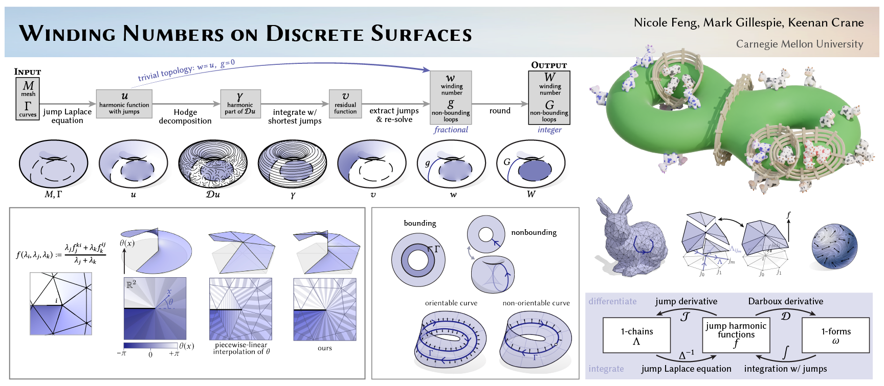
We use \(M\) to denote a surface domain, and \(\Gamma\) some collection of oriented curves on \(M\). As input, the algorithm takes in \(M\) and \(\Gamma\). As output, the algorithm outputs
- an integer labeling of regions bounded by \(\Gamma\)
- a decomposition of \(\Gamma\) into bounding components that induce valid regions vs. nonbounding components
- a closed, completed version of the input curve \(\Gamma\).
As mentioned above, winding number is a jump harmonic function, meaning a function that is harmonic everywhere — including at points on the curve — modulo the jumps. (The function only fails to be harmonic at the curve's endpoints where there is a branch point singularity, shown below.)
Hence our starting point to winding numbers on surfaces is the jump Laplace equation defined on a domain \(M\),
 \[
\begin{align*}
\Delta u &= 0 &\text{on } M\setminus\Gamma\\
u^+ - u^- &= 1^* &\text{on } \Gamma \\
\partial u^+/\partial n &= \partial u^-/\partial n &\text{on } \Gamma
\end{align*}
\]
*More generally, \(u^+(x) - u^-(x) = \) number of times \(\Gamma\) covers \(x\).
\[
\begin{align*}
\Delta u &= 0 &\text{on } M\setminus\Gamma\\
u^+ - u^- &= 1^* &\text{on } \Gamma \\
\partial u^+/\partial n &= \partial u^-/\partial n &\text{on } \Gamma
\end{align*}
\]
*More generally, \(u^+(x) - u^-(x) = \) number of times \(\Gamma\) covers \(x\).
Basically, the jump Laplace equation corresponds to the standard Laplace equation \(\Delta u=0\) (which defines a standard harmonic function), plus a condition that stipulates the solution must jump by a specified integer across the curve \(\Gamma\). Finally, the third equation is a compatibility condition that ensures the solution is indeed harmonic "up to jumps" everywhere on \(M\setminus\partial\Gamma\). Intuitively, for all \(x\notin\Gamma\) the function \(u(x)\) is harmonic in the usual sense, and for \(x\in\Gamma\) (where the jump occurs) it's still possible to locally shift \(u\) such that it once again becomes harmonic in the usual sense (above, right).
Assuming \(M\) is simply-connected, meaning there cannot exist nonbounding loops on \(M\), then we can simply solve the jump Laplace equation above for the function \(u(x)\). If \(\Gamma\) is closed, this case is analogous to ordinary winding number in the plane, which yields a piecewise constant, integer-valued function; every component of \(\Gamma\) is a bounding component.
If \(\Gamma\) is not closed (but \(M\) is still simply-connected), then \(u(x)\) yields a "soft" real-valued (rather than integer-valued) indicator function, analogous to solid angle.
Solving the jump Laplace equation above is Step \(\textcircled{1}\). If \(M\) is not simply-connected, we need to take additional steps. The key insight here is that jump harmonic functions form the "bridge" through which we can transform curves into functions, and vice versa. In particular, jump harmonic functions can both encode curves (where the function jumps in value) as well as a curve's homology class (through its derivative). Our algorithm will amount to a round-trip around the following diagram, where we first translate the input curve \(\Gamma\) into a jump harmonic function, then into a differential 1-form, which you can think of as a vector field. We'll then translate the resulting 1-form back into a jump harmonic function and curve, which will correspond to our final winding number function and curve decomposition, respectively. Performing these translations amounts to using appropriate notions of differentiation and integration.
At a high level, these notions of differentiation and integration simply correspond to their usual notions from ordinary calculus, except we have to take extra care when dealing with the discontinuities of jump harmonic functions. For simplicity, we'll first consider a periodic 1-dimensional function \(f(x)\) defined on the unit interval \([0,1]\):
In general, the gradient of such a function \(f(x)\) with respect to \(x\) yields a continuous part \(\omega:=\mathcal{D}f\), obtained from considering each continuous interval of \(f(x)\), as well as a "jump" part \(\mathcal{J}f\) encoding the location and magnitude of the jumps in \(f(x)\), expressed here as a sum of Dirac-deltas.
For a jump harmonic function in particular, the continuous part \(\omega:=\mathcal{D}f\), which we call the Darboux derivative, "forgets" jumps:
(If you're familiar with differential geometry, you can think of \(\mathcal{D}f\) as "\(df\) modulo jumps", where \(d\) denotes the standard exterior derivative. Just as the standard exterior derivative \(df\) measures the failure of \(f\) to be constant, \(\mathcal{D}f\) measures the failure of \(f\) to be piecewise constant.) In essence, even though jump harmonic functions have discontinuities, the condition of harmonicity forces the Darboux derivative of a jump harmonic function to be globally continuous because the derivatives must "match up" across the discontinuity.
Because the Darboux derivative of a jump harmonic function "forgets" the jumps, there is no unique inverse to Darboux differentiation. In particular, we can only integrate "up to jumps": to continue the previous example, both the original jump harmonic function \(f(x)\) and the function \(g(x)\) shown below are valid possibilities of integrating \(\omega\):
The moral of this story is that to map from derivatives back to curves, we can integrate \(\omega\) and choose the jumps. (This choice of jumps is what will allow us to decompose curves into bounding vs. nonbounding components.)
Our understanding of the 1D case more or less extends directly to the 2D case. Instead of a 1D function on a periodic interval, we can, for example, consider a solution \(u(x)\) of the jump Laplace equation on a 2D periodic domain — namely, a torus:
We arrive at Step \(\textcircled{2}\): taking the Darboux derivative of the jump harmonic function obtained in Step \(\textcircled{1}\). The Darboux derivative \(\omega\) of \(u\) is now a 1-form, which can be thought of as a vector field (shown above). If \(\omega=0\), then \(u(x)\) is piecewise constant, meaning that \(u(x)\) is already a valid (piecewise constant) region labeling. Conversely, if \(w\neq 0\), then there are nonbounding components of \(\Gamma\). In particular, nonbounding components of \(\Gamma\) are encoded by the harmonic component \(\gamma\) of the 1-form \(\omega\). More formally, (non)bounding components of \(\Gamma\) correspond to 1-forms (non)congruent to zero in the first cohomology group \(H^1(M)=\rm{ker}(d_1)\setminus\rm{im}(d_0)\).
Luckily for us, extracting the harmonic component of 1-form can be done via Hodge decomposition, which states that our 1-form \(\omega\) can be decomposed as \(\omega=d\alpha+\delta\beta+\gamma\), where \(\gamma\) is the harmonic 1-form we seek to isolate (and the differential forms \(\alpha\) and \(\beta\) are some scalar and vector potentials). So Step \(\textcircled{3}\) amounts to doing Hodge decomposition to extract the harmonic 1-form \(\gamma\).
In summary, we have transformed our original problem of decomposing the input curve into components that can and cannot be explained as region boundaries, into the well-studied problem of decomposing a vector field into components that can and cannot be explained by a potential.
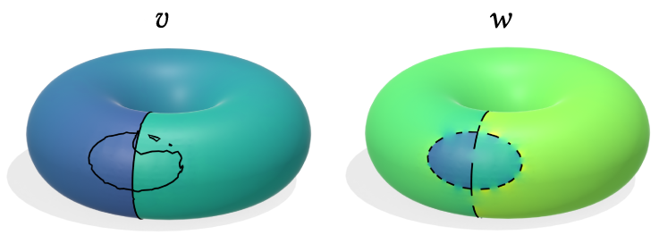
To recap, here is where we are in our round-trip journey so far, using as a visual example a collection of (broken) bounding and nonbounding loops \(\Gamma\) on a torus:
We've used differentiation to obtain a 1-form associated with the original curve \(\Gamma\), then use Hodge decomposition to process this 1-form into a harmonic 1-form \(\gamma\) encoding the nonbounding component of \(\Gamma\). We arrive at Step \(\textcircled{4}\): To determine our curve decomposition, we just have to use integration to translate \(\gamma\) back into a jump harmonic function, and then a curve that will represent the nonbounding component of \(\Gamma\).
More specifically, we search for a scalar potential \(v\) that could have generated \(\gamma\), meaning \(\mathcal{D}v=\gamma\). Since \(\gamma\) is harmonic, \(v\) must jump somewhere; but remember, we get to choose these jumps — and we want the jump derivative \(g:=\mathcal{J}v\) to represent the nonbounding component of \(\Gamma\). We formulate the following optimization that does just this:
In words, the first constraint \(\mathcal{D}v=\gamma\) stipulates that the solution \(v\) should integrate \(\gamma\) in the "Darboux" sense, while the second term in the objective function encourages the jumps \(g=\mathcal{J}v\) in \(v\) to concentrate on a subset of the original curve \(\Gamma\). In the case that \(\Gamma\) is a broken curve, the first term in the objective function also encourages \(g=\mathcal{J}v\) (which necessarily must form closed loops, since \(\gamma\) is harmonic and thus not globally integrable) to be a shortest closed-curve completion of the nonbounding components of \(\Gamma\). Finally, the second constraint discourages spurious extraneous loops in the case that \(\Gamma\) contains multiple nonbounding components of the same homology class.
The solution of this optimization yields a so-called "residual function" \(v\) such that the solution \(w\) to a jump Laplace equation using the curve \(\Gamma - \mathcal{J}v\) is our final winding number function. In other words, we solve for the function \(w\) for which we have removed the influence of \(\Gamma\)'s nonbounding components.
Step \(\textcircled{5}\) is simply reading off the curve decomposition from the residual function \(v\). The locus of points \(\mathcal{J}v\) where \(v\) jumps represents a completion \(G\) of the nonbounding components of the input curve \(\Gamma\); the bounding components of \(\Gamma\) are simply the complement of the nonbounding components, taken as a subset of \(\Gamma\). Additionally, the function \(w\) can be rounded to yield integer region labels \(W\). The entire algorithm is summarized in the following diagram:
With our algorithm described, all that remains is to discretize the algorithm.
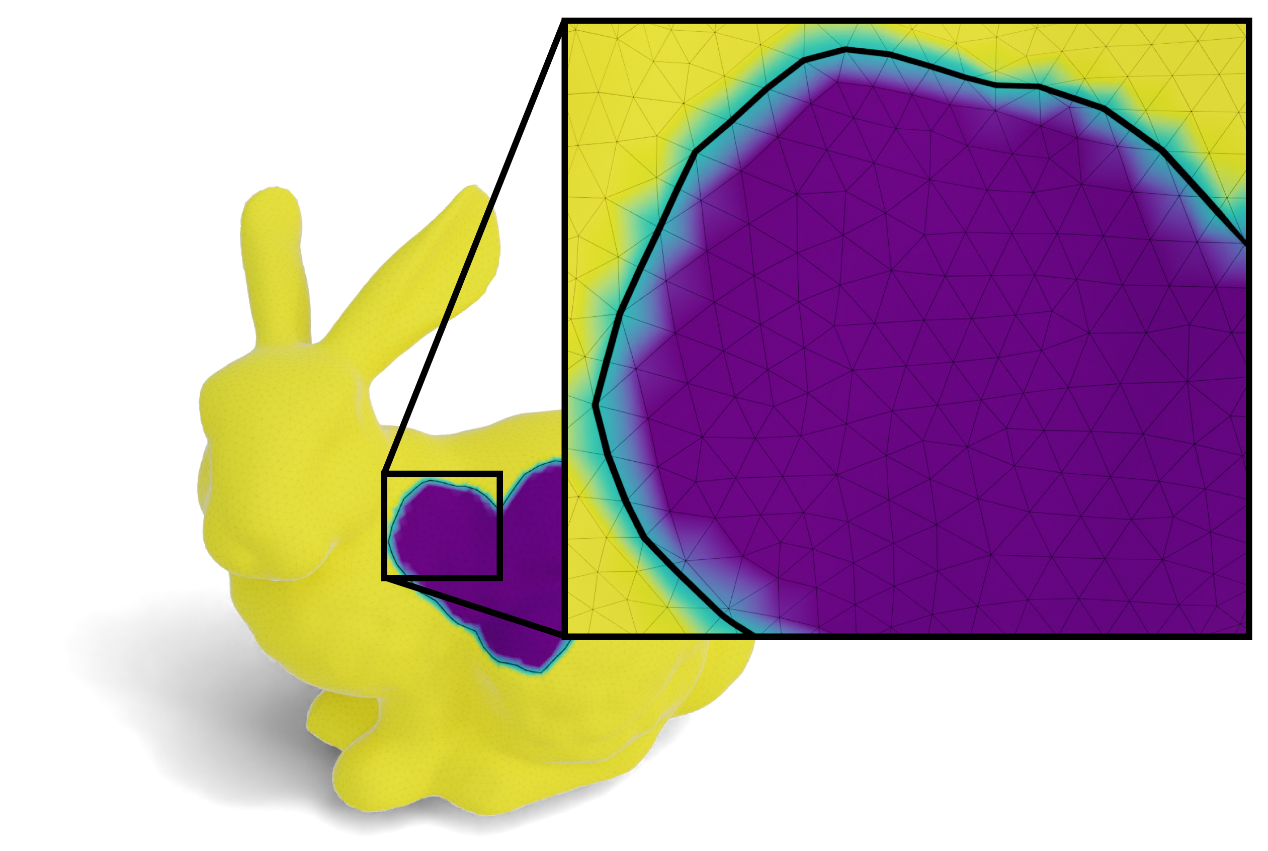
In the discrete setting, we assume the surface domain \(M\) is specified as a triangle mesh. We represent curves and regions as chains on \(M\), meaning as signed integer-value functions on mesh edges and mesh faces, respectively. The jump Laplace equation can be discretized on the mesh as a sparse, positive definite linear system. Performing Hodge decomposition on the gradient of the solution \(u\) amounts to solving another Laplace-type sparse linear system. Finally, performing the integration procedure necessary to map the decomposition of our 1-form to a decomposition of our curve amounts to solving sparse linear program. (The last two steps are only necessary if \(M\) is topologically nontrivial.) For more details, check out our paper, which also contains detailed pseudocode, or our code repository.
Discussion
Commentary that didn't fit in the paper! This section is "for experts only": this section discusses finer technical details, and you certainly don't need to understand this section to understand the paper.
What if the curve isn't constrained to mesh edges?
Our algorithm assumes the input curve \(\Gamma\) is restricted to mesh edges. Can we relax this assumption?
We can: Instead of a Laplace equation with jump conditions, we may consider an equivalent Poisson equation with a source term encoding the gradient of an indicator function: \[\Delta u = \nabla\cdot N\mu_\Gamma. \] The source term on the right-hand side corresponds to a singular vector field concentrated on \(\Gamma\), where the vectors align with the normals of the input curve. This in fact the perspective taken by the classic Poisson Surface Reconstruction algorithm — which, as noted earlier, is mathematically equivalent to generalized winding number and solid angle. (The source term may also be thought of as a simplicial example of the Dirac-\(\delta\) forms described in Wang & Chern 2021.)
We can discretize this Poisson equation using finite elements, although the solution is inevitably "smeared out" somewhat as a result of being regularized by the choice of function space. (In particular, continuous elements will yield approximation error when trying to represent a discontinuous function.)
We can still take the derivative of this function in the same sense of our original algorithm, and Hodge-decompose. On the other hand, integration is less clean.
A dual formulation
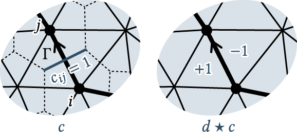
A curve can be viewed as the boundary of "weighted regions", where the weights are the winding numbers. Discretely, this means if we view the curve as a 1-chain \(c\) in a triangulation of the domain, then the winding number is a 2-chain \(b\) such that \(\partial b=c\).
This leads to a "dualized" formulation of the algorithm presented in our paper, where we solve for a dual 0-form (values per face) instead of a primal 0-form. If we encode the curve Γ as a dual 1-chain, then the relationship "Γ bounds a region \(b\)" can be expressed as the linear relation \[db = c\]
where \(d\) is the discrete exterior derivative acting on dual 0-forms, and the jump condition induced by Γ is interpreted as a dual 1-form \(c\).
The least-squares solution is given by another Laplace equation, \[d\ast db = d\ast c.\]
To identify the nonbounding components of the curve, one can do Hodge decomposition on the derivative, just as before (although the corresponding equations will also be appropriately "dualized").
The dual formulation streamlines certain concepts; for example, the "jump derivative" we define in Section 2.4 simply becomes the usual boundary operator (we merely hint at this in Section 3.6.) Encoding the input curve as a dual 1-chain would have also subsumed more difficult situations on non-manifold and non-orientable meshes where primal 1-chains can't unambiguously specify the "sides" of the curve (see discussion in Section 2.2 and 3.7).
The dual algorithm is pretty much the same as the one presented in the paper since it solves the same linear systems and linear program, albeit on dual elements. On the other hand, the primal formulation will perhaps be more familiar to graphics practioners. For example, in the primal formulation, discretizing the jump Laplace equation yields the ordinary cotan-Laplace matrix on vertices, whereas in the dual formulation one would build an analogous cotan-Laplace matrix acting on 2-forms (though the latter isn't any more difficult to build than the former!) You also get better resolution by solving on corners (vertices), rather than on faces.
Conclusion: One approach wasn't clearly better over the other, so we picked the more familiar primal formulation.
$$\newcommand{\assign}[2]{\mathrel{#1}\mathrel{#2}}$$
Hindsights
Reduced-size linear program (~100x speedup)
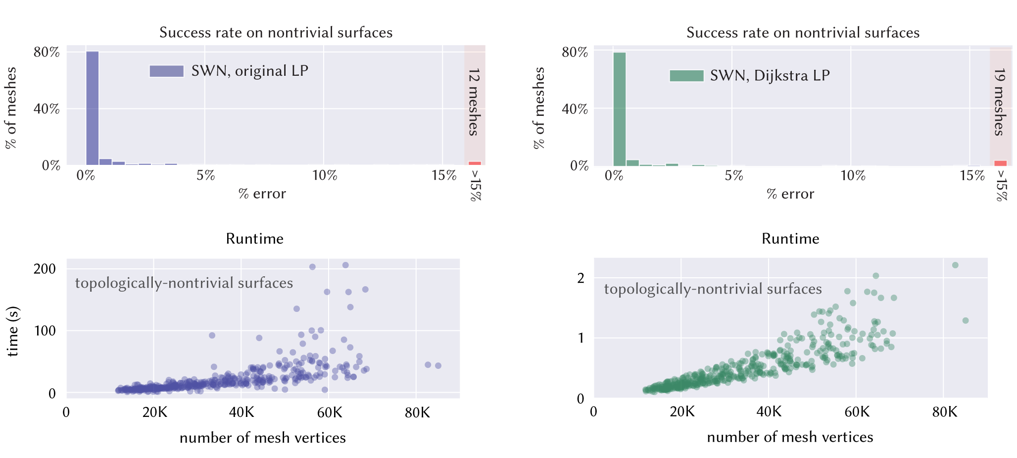
After publication, we realized a simple way to accelerate the linear program optimization in Section 3.4, which results in a ~100x speedup.
The original linear program (LP) simultaneously optimizes for both the sizes and locations of the residual function's jumps. Instead, we could first separately try to complete the curve Γ using a shortest-path heuristic (for example, Dijkstra), partitioning the domain M into several connected components.
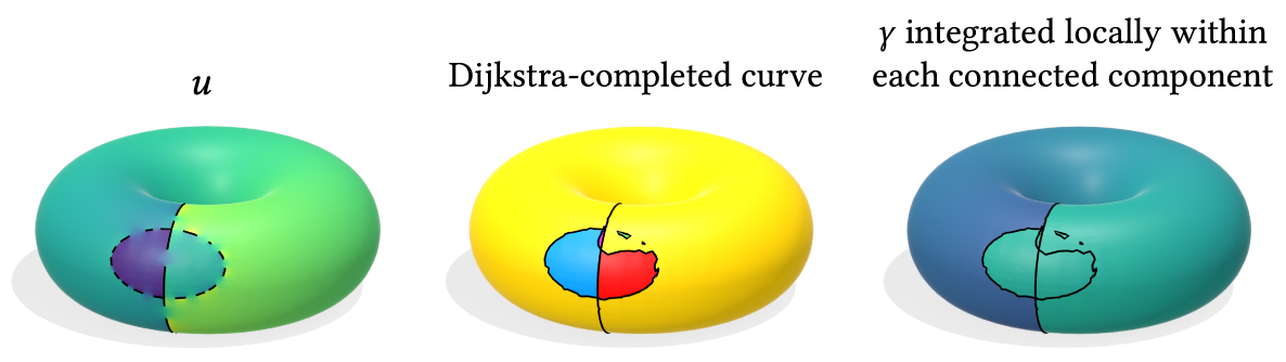
We can locally integrate the harmonic 1-form γ within each connected component — as we did within each triangle face before — before using the original LP to minimize the L1 norm of jumps across connected components.
The number of DOFs is reduced from the number of faces in the mesh to relatively few connected components.
Whereas the original LP took up to a few minutes in the worse cases, this approximate solution takes at most a few seconds, at the cost of a small decrease in accuracy on the benchmark.
We could have also plugged in a different shortest-path method for the curve-completion step; for example, we could use weighted Dijkstra where the weights correspond to the magnitude of the gradient of the jump harmonic function \(u\).
Contouring
Although winding number always produces a nice, visually-intuitive indicator-like function, contouring the winding number is notoriously difficult. My later work on generalized signed distance provides better reconstruction results, no contouring required.
For more on the history of trying to contour the winding number: Jacobson et al. (2013) and Barill et al. (2018) use the 0.5-level set, where the former proposes a graph cut algorithm for more complicated situations. In this project, I found that contouring according to the average value along the input curves to work better, though this still wasn't perfect when multiple curve components were present. Hence this paper presents a contouring procedure that contours according to average shifts to the closest integer.
Errata
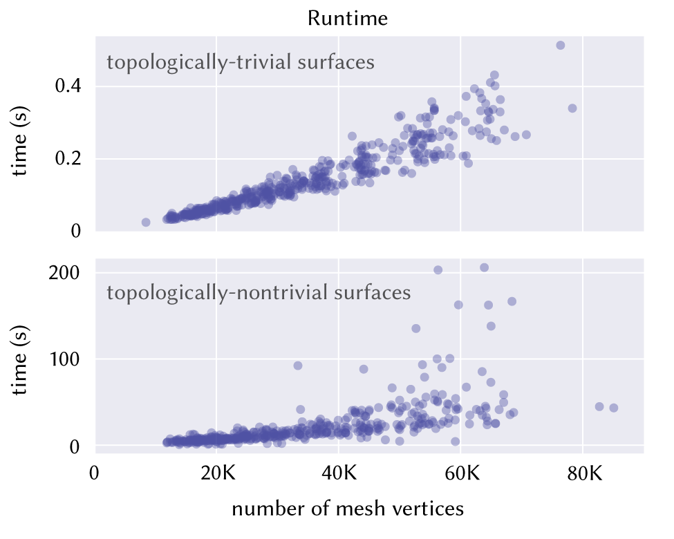
Performance
The runtimes reported in Figure 17 in Section 5.2.2 are inaccurate (something went wrong with job scheduling.) The correct times are ~5x faster when measured on an Intel Xeon W-1250 CPU with 16 GB of RAM (in fact a less powerful processor than the one used in the original paper). The solve times would be even faster using the reduced-size linear program described above in "Hindsights".